State Space Models for Sequence Modelling

State Space Models (SSMs) aim to predict both how inputs into a system are reflected in its outputs and how the state of the system itself evolves over time and in response to specific inputs. SSMs originate from signal and control theory but found uses as a form of “world model” that can process input with reference to information from past inputs to generate the next input.

The state of a system is its internal memory: the information it keeps at time $t$ in order to continue processing the sequence. If the input sequence is

then the state $h_{t}$ is meant to summarize the useful information from everything that has happened so far. In a sequence model, the ideal role of the state is:

This means the model does not need to store the entire past explicitly. Instead, it keeps updating a fixed-size representation as new inputs arrive. The state is used as a compact way to store memory of the previous state and should ideally store useful information from past states while discarding useless information. Since the hidden state is not directly observable, it is a latent state and SSMs are latent models.

An SSM’s method of handling memory can be treated as the opposite of a transformer: while the transformer can look at every single token before the current token to make the next token prediction, an SSM only references the state and current input to produce an output.

The Two Magic Equations

The classical continuous-time state space model is described by two equations:

The state-update equation

The first equation

describes how the hidden state evolves over time based on internal dynamics (hidden state) and the input signal.

• $h(t)$ is the hidden state at time $t$.
• $u(t)$ is the input signal.
• $\dot{h}(t)$ is the derivative of the state, meaning the rate of change of the state.
• $A$ determines how the current state evolves on its own.
• $B$ determines how the new input affects the state.

The output equation

The second equation

describes how the observable output is produced based on the current hidden state (Integrate from $\dot{h}(t)$ obtained previously) and input signal.

• $y(t)$ is the output.
• $C$ reads information from the hidden state.
• $D$ provides a direct path from the input to the output, often interpreted as a skip connection.

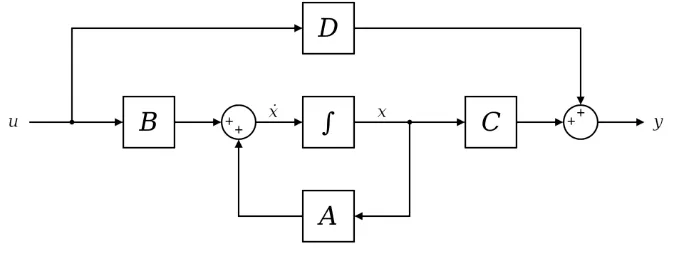
The $B$ block writes the input into the state dynamics, $A$ governs how the state evolves, $C$ reads from the state, and $D$ provides the direct skip path from input to output. Traditional SSMs are continuous-time models meant to model continuous sequences like signals or trajectories which is represented by the diagram above.

However, many data modalities processed by modern deep learning are typically discrete sequences. To use SSM to model a discrete sequence requires a way to represent distinct timesteps as part of a continuous signal. We need a way to update the hidden state as shown below:

Discretization

Discretization amounts to sampling “snapshots” of the value of a continuous function at specific moments. Step size is introduced to determine how long that snapshot is held at each discrete time step. Common discretization methods include Euler’s method and zero order hold which is used in Mamba. Suppose time is divided into steps of size $\Delta$. All continuous changes are summarized into one discrete change within each step.

Euler’s method:

Substituting into the state equation gives:

Rearranging gives:

So the discrete-time matrices become approximately:

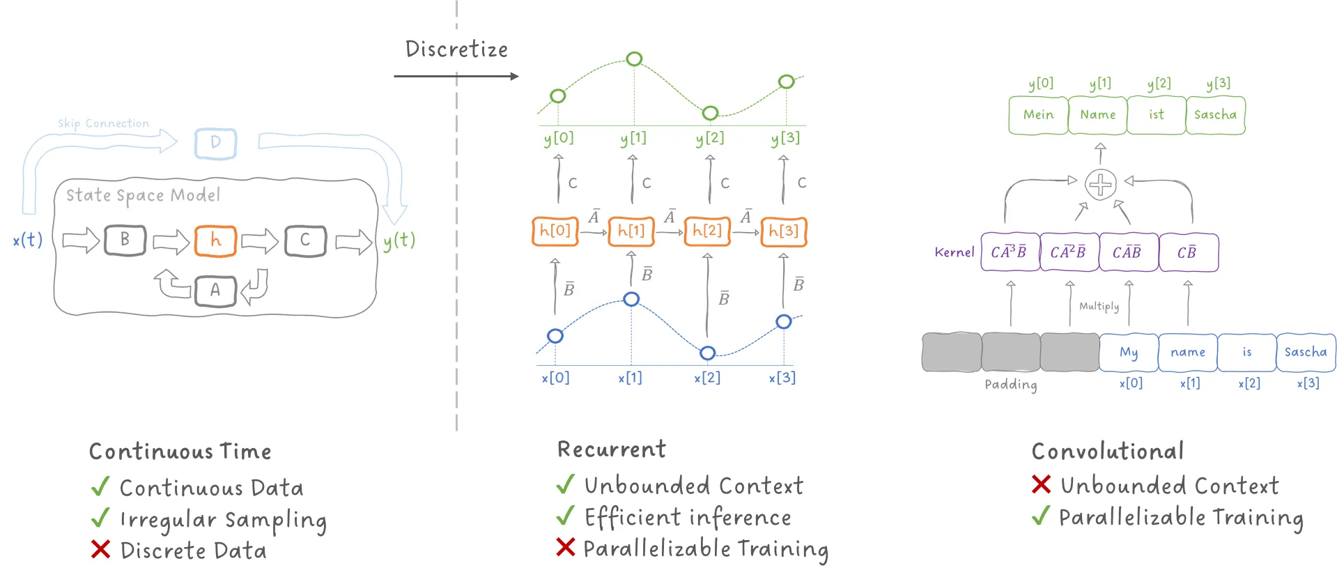
The step size $\Delta$ controls how much continuous-time evolution happens in one discrete step. Small $\Delta$ allows for more fine-grained updates while large $\Delta$ causes more aggressive compression of continuous evolution into each discrete step. Interestingly, discretization introduces 2 new representations of SSMs that are interchangeable: Recurrent and Convolutional.

Recurrent Representation

Once discretized, the SSM takes the form

This is the recurrent representation. Conceptionally, this looks just like a simple RNN where the inputs are processed one at a time, getting combined into a recurrent hidden state and processed to give an output.

At every time step:

1. take the previous hidden state $h_{t - 1}$,
2. update it using the new input $x_{t}$,
3. produce an output $y_{t}$.

Advantages of the recurrent representation

Efficient inference: This is the main selling point of the recurrent representation. At inference time, the model only needs the current hidden state rather than the entire past sequence. This makes it memory efficient when generating or processing inputs one step at a time.

Unbounded context in principle: Because the state keeps evolving, the model can in principle carry information forward indefinitely. The sequence length is not explicitly capped by a fixed context window in the way a pure finite convolution kernel is.

Disadvantages of the recurrent representation

Sequential computation, slower training: Each step depends on the previous one, so training is harder to parallelize across time. Even if inference is efficient, step-by-step processing can make training less efficient on modern hardware compared with methods that exploit more parallelism.

Convolution Representation

The same discretized SSM can also be written as a convolution.

Starting from

we can unroll the recurrence. Then the output becomes

This reveals a convolution kernel:

So the sequence output can be written as

This is the convolution representation. Instead of updating the state one step at a time, we view the SSM as defining a convolution kernel over the entire sequence.

Each term

tells us how an input from $k$ steps ago influences the current output.

Advantages of the convolution representation

Parallelizable training: Because convolutions over the full sequence can be computed in parallel, this representation is much more friendly to modern accelerators during training. When the whole sequence is available especially during training, the convolution view is often the more convenient computational form.

Disadvantages of the convolution representation

Less natural, slower inference: If inputs arrive one at a time, the convolution form is less natural than simply updating a hidden state and thus have slower inference time.

Fixed-kernel limitations: The convolution representation depends on a fixed input-independent kernel. This becomes a limitation when we want content-dependent behaviour, which is one of the motivations for Mamba.

Why Switching Between the Two Views Matters: LSSL

A major insight in modern SSM work is that the same state-space system has three useful views:

1. Continuous-time view — useful for modelling dynamics and irregular sampling.
2. Recurrent view — useful for efficient inference.
3. Convolution view — useful for parallelizable training.

This idea is central to Linear State-Space Layers (LSSL). LSSL showed that a state-space model can be turned into a practical neural sequence layer by moving between these equivalent forms.

The same underlying model can enjoy advantages usually associated with different modelling families:

• good training from the convolutional view,
• good inference from the recurrent view.

The $\mathbf{A}$ Matrix

Among all the matrices in an SSM, the state matrix $A$ is especially important.

In continuous time:

$A$ determines how the hidden state evolves even before considering the new input.

In discrete time:

$\bar{A}$ determines how the previous state is carried into the new one.

So intuitively, $A$ governs the model’s memory dynamics. Repeated application of $\bar{A}$ determines how information from the past survives over time.

From the convolution form,

we can see that older inputs are affected by higher powers of $\bar{A}$.

So the design of $A$ determines whether the model:

• forgets too quickly,
• remembers for a long time,
• captures several timescales,
• represents oscillatory or structured patterns.

A poor choice of $A$ can make the model bad at long-range dependencies. A good choice of $A$ can give the model strong and stable memory. The follow-up question is whether there is a way to design A such that models using these matrices have better memory. Sure enough, some folks at Stanford came up with a general framework known as High-order Polynomial Projection Operator (HiPPO).

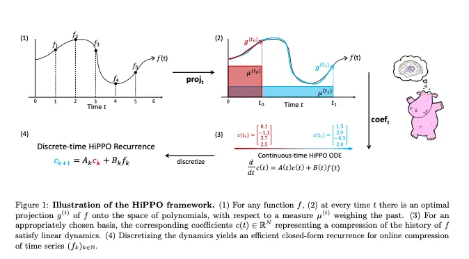
HiPPO is a method for constructing state dynamics so that the hidden state represents a compressed approximation of the past signal. Instead of treating the state as an arbitrary vector, HiPPO gives it a principled interpretation: the state stores coefficients of a compressed representation of the history.

Intuitively, HiPPO matrices are able to retain useful information from more recent states and compress old information. Based on empirical evidence (E.g. S4 paper), HiPPO provides a more meaningful and effective choice of memory dynamics, especially through the $A$ matrix. SSMs perform much better using HiPPO matrix than some random matrix.

Anyone who is good in ODEs can consider looking into the nitty-gritty of HiPPO and contributing a write-up on it. Here is the diagram from the paper to hopefully spark interest (they use a Hippo in the paper):

Structured State Space Sequence Model (S4)

S4’s main significance is that it made SSMs practical for long-sequence deep learning. It was first introduced in 2022 and generated excitement since the architecture is different from CNNs and Transformers (Same year ChatGPT took the world by storm).

S4 can be thought of combining LSSL with HiPPO matrices to produce a stronger SSM that is trainable, good at inference and have good performance thanks to math wizardry. S4’s additional contribution is addressing the issue of matrix A being dense: Generating terms for the convolutional representation will get expensive if A is dense. If the state has dimension N, a dense A matrix has $N^2$ entries.

S4 gives A structured form

S4 tries to make the A matrix easier to compute by expressing A using a diagonal part and a low-rank correction. The diagonal part is written as:

Diagonal matrices are easy to work with because each state dimension evolves independently. If A were purely diagonal, then applying A repeatedly is simple:

This means each hidden-state dimension behaves like its own memory mode. Some modes can decay quickly, some can decay slowly, and some can represent oscillatory behaviour. The model then combines these modes to produce the final output. Different eigenvalues correspond to different memory behaviours where small magnitudes forget quickly, magnitudes near one preserve information longer and complex values can represent oscillations or repeating patterns.

A purely diagonal matrix is efficient, but it can be too restrictive because each dimension evolves independently. The low-rank term

adds a small amount of richer interaction between state dimensions. It is not as expensive as a full dense matrix, but it gives more expressive power than a purely diagonal matrix.

This is the main idea behind the structured matrix:

A = easy diagonal dynamics + small low-rank correction

Limitations of S4

S4 is still mostly based on fixed dynamics. The same state update rule is applied throughout the sequence:

This fixed behaviour is what allows the convolution kernel to exist. However, it also means the model does not directly change its memory rule based on the content of the current input. This becomes a problem for information-dense sequences like language. Sometimes the model should strongly remember a token. Sometimes it should ignore a token. Sometimes it should overwrite old information. A fixed SSM kernel does not naturally provide this kind of content-dependent control.

S5 and Mamba

This section is more to introduce the future developments in the field of SSM for anyone who want to learn more about SSMs. Developments from here onwards are complicated enough to warrant their own articles. After S4, Simplified State Space Layers for Sequence Modeling (S5) is introduced. It can be understood as a cleaner and more scalable version of the structured SSM idea.

In S4-style models, the model often uses many separate single-input, single-output SSMs. Conceptually, each channel of the neural network can have its own SSM. This works, but it is slightly awkward because modern neural networks usually operate on feature vectors rather than one scalar channel at a time.

S5 changes this by using a multi-input, multi-output formulation, usually shortened to MIMO. Instead of treating each feature channel as having a separate little SSM, S5 lets a whole feature vector enter one shared state-space system and reads a whole feature vector out of it. This makes the SSM layer feel more like a normal deep learning layer. S5 also uses parallel scan algorithms, which I am not knowledgeable about GPUs enough to actually explain them but just know parallelism in this case = faster.

Mamba addresses the issue of the memory rule being mostly fixed. A fixed SSM compresses the sequence through a learned state update but the compression is mostly the same across positions. Mamba introduces selective state-space modelling where instead of applying the same memory rule to every input, let the current input influence how memory is updated.

The model can learn to decide whether the token should be written strongly into the state, mostly ignored, used to preserve old memory or used to overwrite previous information. It allows for different sequence elements to be treated differently. Think of selective compression as the compromise between previous iteration’s aggressive compression and transformer expensive lookup of every single past state.